Bose–Einstein statistics

Bose–Einstein statistics apply only to particles that do not follow the Pauli exclusion principle restrictions. Particles that follow Bose-Einstein statistics are called bosons, which have integer values of spin. In contrast, particles that follow Fermi-Dirac statistics are called fermions and have half-integer spins.

Bose–Einstein distribution

At low temperatures, bosons behave differently from fermions (which obey the Fermi–Dirac statistics) in a way that an unlimited number of them can "condense" into the same energy state. This apparently unusual property also gives rise to the special state of matter – the Bose–Einstein condensate. Fermi–Dirac and Bose–Einstein statistics apply when quantum effects are important and the particles are "indistinguishable". Quantum effects appear if the concentration of particles satisfies $\frac{N}{V} \geq n_{q},$ where N is the number of particles, V is the volume, and n_q is the quantum concentration, for which the interparticle distance is equal to the thermal de Broglie wavelength, so that the wavefunctions of the particles are barely overlapping.

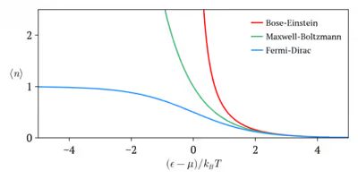
Fermi–Dirac statistics applies to fermions (particles that obey the Pauli exclusion principle), and Bose–Einstein statistics applies to bosons. As the quantum concentration depends on temperature, most systems at high temperatures obey the classical (Maxwell–Boltzmann) limit, unless they also have a very high density, as for a white dwarf. Both Fermi–Dirac and Bose–Einstein become Maxwell–Boltzmann statistics at high temperature or at low concentration.

Bose–Einstein statistics was introduced for photons in 1924 by Bose and generalized to atoms by Einstein in 1924–25.

The expected number of particles in an energy state i for Bose–Einstein statistics is:

${\bar{n}}_{i} = \frac{g_{i}}{e^{(ε_{i} - μ) / k_{B} T} - 1}$

with ε_i > μ and where n_i is the occupation number (the number of particles) in state i, $g_{i}$ is the degeneracy of energy level i, ε_i is the energy of the ith state, μ is the chemical potential (zero for a photon gas), k_B is the Boltzmann constant, and T is the absolute temperature.

The variance of this distribution $V (n)$ is calculated directly from the expression above for the average number. $V (n) = k T \frac{\partial}{\partial μ} {\bar{n}}_{i} = ⟨ n ⟩ (1 + ⟨ n ⟩) = \bar{n} + {\bar{n}}^{2}$

For comparison, the average number of fermions with energy $ε_{i}$ given by Fermi–Dirac particle-energy distribution has a similar form: ${\bar{n}}_{i} (ε_{i}) = \frac{g_{i}}{e^{(ε_{i} - μ) / k_{B} T} + 1} .$

As mentioned above, both the Bose–Einstein distribution and the Fermi–Dirac distribution approaches the Maxwell–Boltzmann distribution in the limit of high temperature and low particle density, without the need for any ad hoc assumptions:

In the limit of low particle density, ${\bar{n}}_{i} = \frac{g_{i}}{e^{(ε_{i} - μ) / k_{B} T} \pm 1} ≪ 1$ , therefore $e^{(ε_{i} - μ) / k_{B} T} \pm 1 ≫ 1$ or equivalently $e^{(ε_{i} - μ) / k_{B} T} ≫ 1$ . In that case, ${\bar{n}}_{i} \approx \frac{g_{i}}{e^{(ε_{i} - μ) / k_{B} T}} = \frac{1}{Z} e^{- (ε_{i} - μ) / k_{B} T}$ , which is the result from Maxwell–Boltzmann statistics.
In the limit of high temperature, the particles are distributed over a large range of energy values, therefore the occupancy on each state (especially the high energy ones with $ε_{i} - μ ≫ k_{B} T$ ) is again very small, ${\bar{n}}_{i} = \frac{g_{i}}{e^{(ε_{i} - μ) / k_{B} T} \pm 1} ≪ 1$ . This again reduces to Maxwell–Boltzmann statistics.

In addition to reducing to the Maxwell–Boltzmann distribution in the limit of high $T$ and low density, Bose–Einstein statistics also reduces to Rayleigh–Jeans law distribution for low energy states with $ε_{i} - μ ≪ k_{B} T$ , namely $\begin{matrix} {\bar{n}}_{i} & = \frac{g_{i}}{e^{(ε_{i} - μ) / k_{B} T} - 1} \\ \approx \frac{g_{i}}{(ε_{i} - μ) / k_{B} T} = \frac{g_{i} k_{B} T}{ε_{i} - μ} . \end{matrix}$

3 more chapters are free with a Lably account.

History

In 1900, Max Planck derived the Planck law to explain blackbody radiation. For this purpose, he introduced the concept of quanta of energy.

Władysław Natanson in 1911 concluded that Planck's law requires indistinguishability of "units of energy", although he did not frame this in terms of Einstein's light quanta.

While presenting a lecture at the University of Dhaka (in what was then British India and is now Bangladesh) on the theory of radiation and the ultraviolet catastrophe, Satyendra Nath Bose intended to show his students that the contemporary theory was inadequate, because it predicted results not in accordance with experimental results. During this lecture, Bose committed an error in applying the theory, which unexpectedly gave a prediction that agreed with the experiment. The error was a simple mistake – similar to arguing that flipping two fair coins will produce two heads one-third of the time – that would appear obviously wrong to anyone with a basic understanding of statistics (remarkably, this error resembled the famous blunder by Jean le Rond d'Alembert known from his Croix ou Pile article). However, the results it predicted agreed with experiment, and Bose realized it might not be a mistake after all. For the first time, he took the position that the Maxwell–Boltzmann distribution would not be true for all microscopic particles at all scales. Thus, he studied the probability of finding particles in various states in phase space, where each state is a little patch having phase volume of h³, and the position and momentum of the particles are not kept particularly separate but are considered as one variable.

Bose adapted this lecture into a short article called "Planck's law and the hypothesis of light quanta" and submitted it to the Philosophical Magazine. However, the referee's report was negative, and the paper was rejected. Undaunted, he sent the manuscript to Albert Einstein requesting publication in the Zeitschrift für Physik. Einstein immediately agreed, personally translated the article from English into German (Bose had earlier translated Einstein's article on the general theory of relativity from German to English), and saw to it that it was published. Bose's theory achieved respect when Einstein sent his own paper in support of Bose's to Zeitschrift für Physik, asking that they be published together. The paper came out in 1924.

The reason Bose produced accurate results was that since photons are indistinguishable from each other, one cannot treat any two photons having equal quantum numbers (e.g., polarization and momentum vector) as being two distinct identifiable photons. Bose originally had a factor of 2 for the possible spin states, but Einstein changed it to polarization. By analogy, if in an alternate universe coins were to behave like photons and other bosons, the probability of producing two heads would indeed be one-third, and so is the probability of getting a head and a tail which equals one-half for the conventional (classical, distinguishable) coins. Bose's "error" leads to what is now called Bose–Einstein statistics.

Bose and Einstein extended the idea to atoms and this led to the prediction of the existence of phenomena which became known as Bose–Einstein condensate, a dense collection of bosons (which are particles with integer spin, named after Bose), which was demonstrated to exist by experiment in 1995.

Derivation

Derivation from the microcanonical ensemble

In the microcanonical ensemble, one considers a system with fixed energy, volume, and number of particles. We take a system composed of $N = \sum_{i} n_{i}$ identical bosons, $n_{i}$ of which have energy $ε_{i}$ and are distributed over $g_{i}$ levels or states with the same energy $ε_{i}$ , i.e. $g_{i}$ is the degeneracy associated with energy $ε_{i}$ . The total energy of the system is $E = \sum_{i} n_{i} ε_{i}$ . Calculation of the number of arrangements of $n_{i}$ particles distributed among $g_{i}$ states is a problem of combinatorics. Since particles are indistinguishable in the quantum mechanical context here, the number of ways for arranging $n_{i}$ particles in $g_{i}$ boxes (for the $i$ th energy level), where each box is capable of containing an infinite number of bosons (because for bosons the Pauli exclusion principle does not apply), would be (see image):

$w_{i, BE} = \frac{(n_{i} + g_{i} - 1)!}{n_{i}! (g_{i} - 1)!} = C_{n_{i}}^{n_{i} + g_{i} - 1},$ where $C_{k}^{m}$ is the k-combination of a set with m elements (Note also that $w_{i, BE}$ represents the absolute non-normalized probability of an energy state with $n_{i}$ bosons and a degeneracy of $g_{i}$ , it is not the same as the $w_{i}$ associated with the Gibbs formulation of entropy). The total number of arrangements in an ensemble of bosons is simply the product of the binomial coefficients $C_{n_{i}}^{n_{i} + g_{i} - 1}$ above over all the energy levels, i.e. $W_{BE} = \prod_{i} w_{i, BE} = \prod_{i} \frac{(n_{i} + g_{i} - 1)!}{(g_{i} - 1)! n_{i}!},$

which for very large $n_{i}$ and $g_{i}$ can be simplified using Stirling's approximation to

$W_{BE} = \prod_{i} \frac{(\frac{n_{i} + g_{i} - 1}{e})^{n_{i} + g_{i} - 1}}{(\frac{g_{i} - 1}{e})^{g_{i} - 1} (\frac{n_{i}}{e})^{n_{i}}} .$

The entropy of the system can then be expressed as

$S_{BE} = k_{B} ln W_{BE} = k_{B} \sum_{i} [(n_{i} + g_{i} - 1) (ln (n_{i} + g_{i} - 1) - 1) - (g_{i} - 1) (ln (g_{i} - 1) - 1) - n_{i} (ln n_{i} - 1)] .$

The three constraints we can impose on the system can be expressed as

$\sum_{i} δ n_{i} = 0$

(conservation of N),

$\sum_{i} ϵ_{i} δ n_{i} = 0$

(conservation of E), and

$δ S_{BE} = 0$

(second law of thermodynamics for a system at equilibrium).

This final constraint can be expanded to be in terms of $n_{i}$ :

$δ S_{BE} = \frac{\partial}{\partial n_{i}} S_{BE} δ n_{i} = k_{B} \sum_{i} [ln (n_{i} + g_{i} - 1) - ln n_{i}] δ n_{i} = 0.$

Now we can write

$\sum_{i} [ln (n_{i} + g_{i} - 1) - ln n_{i}] δ n_{i} + C \sum_{i} δ n_{i} - β \sum_{i} ϵ_{i} δ n_{i} = 0,$

for which to be true, it must be the case that for any i

$ln (n_{i} + g_{i} - 1) - ln n_{i} + C - β ϵ_{i} = 0.$

By solving for $n_{i}$ and simplifying we obtain

$n_{i} = \frac{g_{i} - 1}{α e^{β ϵ_{i}} - 1},$

which for sufficiently large $g_{i}$ reduces to

$n_{i} = \frac{g_{i}}{α e^{β ϵ_{i}} - 1},$

which is the form of the Bose-Einstein distribution. Note that this form holds even for a system of interacting bosons.

Derivation from the grand canonical ensemble

The Bose–Einstein distribution, which applies only to a quantum system of non-interacting bosons, is naturally derived from the grand canonical ensemble without any approximations. In this ensemble, the system is able to exchange energy and exchange particles with a reservoir (temperature T and chemical potential μ fixed by the reservoir).

Due to the non-interacting quality, each available single-particle level (with energy level ϵ) forms a separate thermodynamic system in contact with the reservoir. That is, the number of particles within the overall system that occupy a given single particle state form a sub-ensemble that is also grand canonical ensemble; hence, it may be analysed through the construction of a grand partition function.

Every single-particle state is of a fixed energy, $ε$ . As the sub-ensemble associated with a single-particle state varies by the number of particles only, it is clear that the total energy of the sub-ensemble is also directly proportional to the number of particles in the single-particle state; where $N$ is the number of particles, the total energy of the sub-ensemble will then be $N ε$ . Beginning with the standard expression for a grand partition function and replacing $E$ with $N ε$ , the grand partition function takes the form $Z = \sum_{N} \exp ((N μ - N ε) / k_{B} T) = \sum_{N} \exp (N (μ - ε) / k_{B} T)$

This formula applies to fermionic systems as well as bosonic systems. Fermi–Dirac statistics arises when considering the effect of the Pauli exclusion principle: whilst the number of fermions occupying the same single-particle state can only be either 1 or 0, the number of bosons occupying a single particle state may be any integer. Thus, the grand partition function for bosons can be considered a geometric series and may be evaluated as such: $\begin{matrix} Z & = \sum_{N = 0}^{\infty} \exp (N (μ - ε) / k_{B} T) = \sum_{N = 0}^{\infty} [\exp ((μ - ε) / k_{B} T)]^{N} \\ = \frac{1}{1 - \exp ((μ - ε) / k_{B} T)} . \end{matrix}$

Note that the geometric series is convergent only if $e^{(μ - ε) / k_{B} T} < 1$ , including the case where $ε = 0$ . This implies that the chemical potential for the Bose gas must be negative, i.e., $μ < 0$ , whereas the Fermi gas is allowed to take both positive and negative values for the chemical potential.

The average particle number for that single-particle substate is given by $⟨ N ⟩ = k_{B} T \frac{1}{Z} {(\frac{\partial Z}{\partial μ})}_{V, T} = \frac{1}{\exp ((ε - μ) / k_{B} T) - 1}$ This result applies for each single-particle level and thus forms the Bose–Einstein distribution for the entire state of the system.

The variance in particle number, $σ_{N}^{2} = ⟨ N^{2} ⟩ - ⟨ N ⟩^{2}$ , is: $σ_{N}^{2} = k_{B} T {(\frac{d ⟨ N ⟩}{d μ})}_{V, T} = \frac{\exp ((ε - μ) / k_{B} T)}{(\exp ((ε - μ) / k_{B} T) - 1)^{2}} = ⟨ N ⟩ (1 + ⟨ N ⟩) .$

As a result, for highly occupied states the standard deviation of the particle number of an energy level is very large, slightly larger than the particle number itself: $σ_{N} \approx ⟨ N ⟩$ . This large uncertainty is due to the fact that the probability distribution for the number of bosons in a given energy level is a geometric distribution; somewhat counterintuitively, the most probable value for N is always 0. (In contrast, classical particles have instead a Poisson distribution in particle number for a given state, with a much smaller uncertainty of $σ_{N, c l a s s i c a l} = \sqrt{⟨ N ⟩}$ , and with the most-probable N value being near $⟨ N ⟩$ .)

Derivation in the canonical approach

It is also possible to derive approximate Bose–Einstein statistics in the canonical ensemble. These derivations are lengthy and only yield the above results in the asymptotic limit of a large number of particles. The reason is that the total number of bosons is fixed in the canonical ensemble. The Bose–Einstein distribution in this case can be derived as in most texts by maximization, but the mathematically best derivation is by the Darwin–Fowler method of mean values as emphasized by Dingle. See also Müller-Kirsten. The fluctuations of the ground state in the condensed region are however markedly different in the canonical and grand-canonical ensembles.

Interdisciplinary applications

Viewed as a pure probability distribution, the Bose–Einstein distribution has found application in other fields:

In recent years, Bose–Einstein statistics has also been used as a method for term weighting in information retrieval. The method is one of a collection of DFR ("Divergence From Randomness") models, the basic notion being that Bose–Einstein statistics may be a useful indicator in cases where a particular term and a particular document have a significant relationship that would not have occurred purely by chance. Source code for implementing this model is available from the Terrier project at the University of Glasgow.
The evolution of many complex systems, including the World Wide Web, business, and citation networks, is encoded in the dynamic web describing the interactions between the system's constituents. Despite their irreversible and nonequilibrium nature these networks follow Bose statistics and can undergo Bose–Einstein condensation. Addressing the dynamical properties of these nonequilibrium systems within the framework of equilibrium quantum gases predicts that the "first-mover-advantage", "fit-get-rich" (FGR) and "winner-takes-all" phenomena observed in competitive systems are thermodynamically distinct phases of the underlying evolving networks.