Holonomy · Lablypedia

Any kind of connection on a manifold gives rise, through its parallel transport maps, to some notion of holonomy. The most common forms of holonomy are for connections possessing some kind of symmetry. Important examples include: holonomy of the Levi-Civita connection in Riemannian geometry (called Riemannian holonomy), holonomy of connections in vector bundles, holonomy of Cartan connections, and holonomy of connections in principal bundles. In each of these cases, the holonomy of the connection can be identified with a Lie group, the holonomy group. The holonomy of a connection is closely related to the curvature of the connection, via the Ambrose–Singer theorem.

The study of Riemannian holonomy has led to a number of important developments. Holonomy was introduced by Élie Cartan (1926) in order to study and classify symmetric spaces. It was not until much later that holonomy groups would be used to study Riemannian geometry in a more general setting. In 1952 Georges de Rham proved the de Rham decomposition theorem, a principle for splitting a Riemannian manifold into a Cartesian product of Riemannian manifolds by splitting the tangent bundle into irreducible spaces under the action of the local holonomy groups. Later, in 1953, Marcel Berger classified the possible irreducible holonomies. The decomposition and classification of Riemannian holonomy has applications to physics and to string theory.

Definitions

Holonomy of a connection in a vector bundle

Let E be a rank-k vector bundle over a smooth manifold M, and let ∇ be a connection on E. Given a piecewise smooth loop γ : [0,1] → M based at x in M, the connection defines a parallel transport map P_γ : E_x → E_x on the fiber of E at x. This map is both linear and invertible, and so defines an element of the general linear group GL(E_x). The holonomy group of ∇ based at x is defined as

{Hol}_{x} (\nabla) = {P_{γ} \in G L (E_{x}) ∣ γ is a loop based at x} .

The restricted holonomy group based at x is the subgroup ${Hol}_{x}^{0} (\nabla)$ coming from contractible loops γ.

If M is path-connected, then the holonomy group depends on the basepoint x only up to conjugation in GL(k, R). Explicitly, if γ is a path from x to y in M, then

{Hol}_{y} (\nabla) = P_{γ} {Hol}_{x} (\nabla) P_{γ}^{- 1} .

Choosing different identifications of E_x with R^k also gives conjugate subgroups. Sometimes, particularly in general or informal discussions (such as below), one may drop reference to the basepoint, with the understanding that it is defined uniquely only up to conjugation.

Some important properties of the holonomy group include:

${Hol}^{0} (\nabla)$ is a connected Lie subgroup of GL(k, R).
${Hol}^{0} (\nabla)$ is the identity component of $Hol (\nabla) .$
If M is simply connected, then $Hol (\nabla) = {Hol}^{0} (\nabla) .$
∇ is flat (i.e. has vanishing curvature) if and only if ${Hol}^{0} (\nabla)$ is trivial. In this case, $Hol (\nabla)$ may still be nontrivial.
There is a natural, surjective group homomorphism $π_{1} (M) \to Hol (\nabla) / {Hol}^{0} (\nabla),$ where $π_{1} (M)$ is the fundamental group of M, which sends the homotopy class $[γ]$ to the coset $P_{γ} \cdot {Hol}^{0} (\nabla) .$

Holonomy of a connection in a principal bundle

The definition for holonomy of connections on principal bundles proceeds in parallel fashion. Let G be a Lie group and P a principal G-bundle over a smooth manifold M which is paracompact. Let ω be a connection on P. Given a piecewise smooth loop γ : [0,1] → M based at x in M and a point p in the fiber over x, the connection defines a unique horizontal lift $\tilde{γ} : [0, 1] \to P$ such that $\tilde{γ} (0) = p .$ The end point of the horizontal lift, $\tilde{γ} (1)$ , will not generally be p but rather some other point p·g in the fiber over x. Define an equivalence relation ~ on P by saying that p ~ q if they can be joined by a piecewise smooth horizontal path in P.

The holonomy group of ω based at p is then defined as

{Hol}_{p} (ω) = {g \in G ∣ p \sim p \cdot g} .

The restricted holonomy group based at p is the subgroup ${Hol}_{p}^{0} (ω)$ coming from horizontal lifts of contractible loops γ.

If M and P are connected then the holonomy group depends on the basepoint p only up to conjugation in G. Explicitly, if q is any other chosen basepoint for the holonomy, then there exists a unique g ∈ G such that q ~ p·g. With this value of g,

{Hol}_{q} (ω) = g^{- 1} {Hol}_{p} (ω) g .

In particular,

{Hol}_{p \cdot g} (ω) = g^{- 1} {Hol}_{p} (ω) g .

Moreover, if p ~ q then ${Hol}_{p} (ω) = {Hol}_{q} (ω) .$ As above, sometimes one drops reference to the basepoint of the holonomy group, with the understanding that the definition is good up to conjugation.

Some important properties of the holonomy and restricted holonomy groups include:

${Hol}_{p}^{0} (ω)$ is a connected Lie subgroup of G.
${Hol}_{p}^{0} (ω)$ is the identity component of ${Hol}_{p} (ω) .$
There is a natural, surjective group homomorphism $π_{1} \to {Hol}_{p} (ω) / {Hol}_{p}^{0} (ω) .$
If M is simply connected then ${Hol}_{p} (ω) = {Hol}_{p}^{0} (ω) .$
ω is flat (i.e. has vanishing curvature) if and only if ${Hol}_{p}^{0} (ω)$ is trivial.

Holonomy bundles

Let M be a connected paracompact smooth manifold and P a principal G-bundle with connection ω, as above. Let p ∈ P be an arbitrary point of the principal bundle. Let H(p) be the set of points in P which can be joined to p by a horizontal curve. Then it can be shown that H(p), with the evident projection map, is a principal bundle over M with structure group ${Hol}_{p} (ω) .$ This principal bundle is called the holonomy bundle (through p) of the connection. The connection ω restricts to a connection on H(p), since its parallel transport maps preserve H(p). Thus H(p) is a reduced bundle for the connection. Furthermore, since no subbundle of H(p) is preserved by parallel transport, it is the minimal such reduction.

As with the holonomy groups, the holonomy bundle also transforms equivariantly within the ambient principal bundle P. In detail, if q ∈ P is another chosen basepoint for the holonomy, then there exists a unique g ∈ G such that q ~ p g (since, by assumption, M is path-connected). Hence H(q) = H(p) g. As a consequence, the induced connections on holonomy bundles corresponding to different choices of basepoint are compatible with one another: their parallel transport maps will differ by precisely the same element g.

Monodromy

The holonomy bundle H(p) is a principal bundle for ${Hol}_{p} (ω),$ and so also admits an action of the restricted holonomy group ${Hol}_{p}^{0} (ω)$ (which is a normal subgroup of the full holonomy group). The discrete group ${Hol}_{p} (ω) / {Hol}_{p}^{0} (ω)$ is called the monodromy group of the connection; it acts on the quotient bundle $H (p) / {Hol}_{p}^{0} (ω) .$ There is a surjective homomorphism $φ : π_{1} \to {Hol}_{p} (ω) / {Hol}_{p}^{0} (ω),$ so that $φ (π_{1} (M))$ acts on $H (p) / {Hol}_{p}^{0} (ω) .$ This action of the fundamental group is a monodromy representation of the fundamental group.

Local and infinitesimal holonomy

If π: P → M is a principal bundle, and ω is a connection in P, then the holonomy of ω can be restricted to the fibre over an open subset of M. Indeed, if U is a connected open subset of M, then ω restricts to give a connection in the bundle π⁻¹U over U. The holonomy (resp. restricted holonomy) of this bundle will be denoted by ${Hol}_{p} (ω, U)$ (resp. ${Hol}_{p}^{0} (ω, U)$ ) for each p with π(p) ∈ U.

If U ⊂ V are two open sets containing π(p), then there is an evident inclusion

{Hol}_{p}^{0} (ω, U) \subset {Hol}_{p}^{0} (ω, V) .

The local holonomy group at a point p is defined by

{Hol}^{*} (ω) = ⋂_{k = 1}^{\infty} {Hol}^{0} (ω, U_{k})

for any family of nested connected open sets U_k with $⋂_{k} U_{k} = π (p)$ .

The local holonomy group has the following properties:

It is a connected Lie subgroup of the restricted holonomy group ${Hol}_{p}^{0} (ω) .$
Every point p has a neighborhood V such that ${Hol}_{p}^{*} (ω) = {Hol}_{p}^{0} (ω, V) .$ In particular, the local holonomy group depends only on the point p, and not the choice of sequence U_k used to define it.
The local holonomy is equivariant with respect to translation by elements of the structure group G of P; i.e., ${Hol}_{p g}^{*} (ω) = Ad (g^{- 1}) {Hol}_{p}^{*} (ω)$ for all g ∈ G. (Note that, by property 1, the local holonomy group is a connected Lie subgroup of G, so the adjoint is well-defined.)

The local holonomy group is not well-behaved as a global object. In particular, its dimension may fail to be constant. However, the following theorem holds:

If the dimension of the local holonomy group is constant, then the local and restricted holonomy agree:

{Hol}_{p}^{*} (ω) = {Hol}_{p}^{0} (ω) .

4 more chapters are free with a Lably account.

Ambrose–Singer theorem

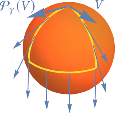
The Ambrose–Singer theorem (due to Warren Ambrose and Isadore M. Singer (1953)) relates the holonomy of a connection in a principal bundle with the curvature form of the connection. To make this theorem plausible, consider the familiar case of an affine connection (or a connection in the tangent bundle – the Levi-Civita connection, for example). The curvature arises when one travels around an infinitesimal parallelogram.

In detail, if σ: [0, 1] × [0, 1] → M is a surface in M parametrized by a pair of variables x and y, then a vector V may be transported around the boundary of σ: first along (x, 0), then along (1, y), followed by (x, 1) going in the negative direction, and then (0, y) back to the point of origin. This is a special case of a holonomy loop: the vector V is acted upon by the holonomy group element corresponding to the lift of the boundary of σ. The curvature enters explicitly when the parallelogram is shrunk to zero, by traversing the boundary of smaller parallelograms over [0, x] × [0, y]. This corresponds to taking a derivative of the parallel transport maps at x = y = 0:

\frac{D}{d x} \frac{D}{d y} V - \frac{D}{d y} \frac{D}{d x} V = R (\frac{\partial σ}{\partial x}, \frac{\partial σ}{\partial y}) V

where R is the curvature tensor. So, roughly speaking, the curvature gives the infinitesimal holonomy over a closed loop (the infinitesimal parallelogram). More formally, the curvature is the differential of the holonomy action at the identity of the holonomy group. In other words, R(X, Y) is an element of the Lie algebra of ${Hol}_{p} (ω) .$

In general, consider the holonomy of a connection in a principal bundle P → M over P with structure group G. Let g denote the Lie algebra of G, the curvature form of the connection is a g-valued 2-form Ω on P. The Ambrose–Singer theorem states:

The Lie algebra of

{Hol}_{p} (ω)

is spanned by all the elements of g of the form

Ω_{q} (X, Y)

as q ranges over all points which can be joined to p by a horizontal curve (q ~ p), and X and Y are horizontal tangent vectors at q.

Alternatively, the theorem can be restated in terms of the holonomy bundle:

The Lie algebra of

{Hol}_{p} (ω)

is the subspace of g spanned by elements of the form

Ω_{q} (X, Y)

where q ∈ H(p) and X and Y are horizontal vectors at q.

Riemannian holonomy

The holonomy of a Riemannian manifold (M, g) is the holonomy group of the Levi-Civita connection on the tangent bundle to M. A 'generic' n-dimensional Riemannian manifold has an O(n) holonomy, or SO(n) if it is orientable. Manifolds whose holonomy groups are proper subgroups of O(n) or SO(n) have special properties.

One of the earliest fundamental results on Riemannian holonomy is the theorem of Borel & Lichnerowicz (1952), which asserts that the restricted holonomy group is a closed Lie subgroup of O(n). In particular, it is compact.

Reducible holonomy and the de Rham decomposition

Let x ∈ M be an arbitrary point. Then the holonomy group Hol(M) acts on the tangent space T_xM. This action may either be irreducible as a group representation, or reducible in the sense that there is a splitting of T_xM into orthogonal subspaces T_xM = T′_xM ⊕ T″_xM, each of which is invariant under the action of Hol(M). In the latter case, M is said to be reducible.

Suppose that M is a reducible manifold. Allowing the point x to vary, the bundles T′M and T″M formed by the reduction of the tangent space at each point are smooth distributions which are integrable in the sense of Frobenius. The integral manifolds of these distributions are totally geodesic submanifolds. So M is locally a Cartesian product M′ × M″. The (local) de Rham isomorphism follows by continuing this process until a complete reduction of the tangent space is achieved:

Let M be a simply connected Riemannian manifold, and TM = T⁽⁰⁾M ⊕ T⁽¹⁾M ⊕ ⋯ ⊕ T^(k)M be the complete reduction of the tangent bundle under the action of the holonomy group. Suppose that T⁽⁰⁾M consists of vectors invariant under the holonomy group (i.e., such that the holonomy representation is trivial). Then locally M is isometric to a product

V_{0} \times V_{1} \times \dots \times V_{k},

where V₀ is an open set in a Euclidean space, and each V_i is an integral manifold for T⁽ⁱ⁾M. Furthermore, Hol(M) splits as a direct product of the holonomy groups of each M_i, the maximal integral manifold of T⁽ⁱ⁾ through a point.

If, moreover, M is assumed to be geodesically complete, then the theorem holds globally, and each M_i is a geodesically complete manifold.

The Berger classification

In 1955, M. Berger gave a complete classification of possible holonomy groups for simply connected, Riemannian manifolds which are irreducible (not locally a product space) and nonsymmetric (not locally a Riemannian symmetric space). Berger's list is as follows:

Manifolds with holonomy Sp(n)·Sp(1) were simultaneously studied in 1965 by Edmond Bonan and Vivian Yoh Kraines, who both discovered that such manifolds would necessarily carry a parallel 4-form.

Manifolds with holonomy G₂ or Spin(7) were first investigated in abstract by Bonan in 1966, who classified the parallel differential forms that such a manifold would carry, and showed that such a manifold would necessarily be Ricci-flat. However, no examples of such manifolds would actually be constructed for another 30 years.

Berger's original list also included the possibility of Spin(9) as a subgroup of SO(16). Riemannian manifolds with such holonomy were later shown independently by D. Alekseevski and Brown-Gray to be necessarily locally symmetric, i.e., locally isometric to the Cayley plane F₄/Spin(9) or locally flat. See below.) It is now known that all of these possibilities occur as holonomy groups of Riemannian manifolds. The last two exceptional cases were the most difficult to find. See G₂ manifold and Spin(7) manifold.

Note that Sp(n) ⊂ SU(2n) ⊂ U(2n) ⊂ SO(4n), so every hyperkähler manifold is a Calabi–Yau manifold, every Calabi–Yau manifold is a Kähler manifold, and every Kähler manifold is orientable.

The strange list above was explained by Simons's proof of Berger's theorem. A simple and geometric proof of Berger's theorem was given by Carlos E. Olmos in 2005. One first shows that if a Riemannian manifold is not a locally symmetric space and the reduced holonomy acts irreducibly on the tangent space, then it acts transitively on the unit sphere. The Lie groups acting transitively on spheres are known: they consist of the list above, together with 2 extra cases: the group Spin(9) acting on R¹⁶, and the group T · Sp(m) acting on R^4m. Finally one checks that the first of these two extra cases only occurs as a holonomy group for locally symmetric spaces (that are locally isomorphic to the Cayley projective plane), and the second does not occur at all as a holonomy group.

Berger's original classification also included non-positive-definite pseudo-Riemannian metric non-locally symmetric holonomy. That list consisted of SO(p,q) of signature (p, q), U(p, q) and SU(p, q) of signature (2p, 2q), Sp(p, q) and Sp(p, q)·Sp(1) of signature (4p, 4q), SO(n, C) of signature (n, n), SO(n, H) of signature (2n, 2n), split G₂ of signature (4, 3), G₂(C) of signature (7, 7), Spin(4, 3) of signature (4, 4), Spin(7, C) of signature (7,7), Spin(5,4) of signature (8,8) and, lastly, Spin(9, C) of signature (16,16). The split and complexified Spin(9) are necessarily locally symmetric as above and should not have been on the list. The complexified holonomies SO(n, C), G₂(C), and Spin(7,C) may be realized from complexifying real analytic Riemannian manifolds. The last case, manifolds with holonomy contained in SO(n, H), were shown to be locally flat by R. McLean.

Riemannian symmetric spaces, which are locally isometric to homogeneous spaces G/H have local holonomy isomorphic to H. These too have been completely classified.

Finally, Berger's paper lists possible holonomy groups of manifolds with only a torsion-free affine connection; this is discussed below.

Special holonomy and spinors

Manifolds with special holonomy are characterized by the presence of parallel spinors, meaning spinor fields with vanishing covariant derivative. In particular, the following facts hold:

Hol(ω) ⊂ U(n) if and only if M admits a covariantly constant (or parallel) projective pure spinor field.
If M is a spin manifold, then Hol(ω) ⊂ SU(n) if and only if M admits at least two linearly independent parallel pure spinor fields. In fact, a parallel pure spinor field determines a canonical reduction of the structure group to SU(n).
If M is a seven-dimensional spin manifold, then M carries a non-trivial parallel spinor field if and only if the holonomy is contained in G₂.
If M is an eight-dimensional spin manifold, then M carries a non-trivial parallel spinor field if and only if the holonomy is contained in Spin(7).

The unitary and special unitary holonomies are often studied in connection with twistor theory, as well as in the study of almost complex structures.

Applications

String theory

Riemannian manifolds with special holonomy play an important role in string theory compactifications. This is because special holonomy manifolds admit covariantly constant (parallel) spinors and thus preserve some fraction of the original supersymmetry. Most important are compactifications on Calabi–Yau manifolds with SU(2) or SU(3) holonomy. Also important are compactifications on G₂ manifolds.

Machine learning

Computing the holonomy of Riemannian manifolds has been suggested as a way to learn the structure of data manifolds in machine learning, in particular in the context of manifold learning. As the holonomy group contains information about the global structure of the data manifold, it can be used to identify how the data manifold might decompose into a product of submanifolds. The holonomy cannot be computed exactly due to finite sampling effects, but it is possible to construct a numerical approximation using ideas from spectral graph theory similar to Vector Diffusion Maps. The resulting algorithm, the Geometric Manifold Component Estimator (GeoManCEr) gives a numerical approximation to the de Rham decomposition that can be applied to real-world data.

Affine holonomy

Affine holonomy groups are the groups arising as holonomies of torsion-free affine connections; those which are not Riemannian or pseudo-Riemannian holonomy groups are also known as non-metric holonomy groups. The de Rham decomposition theorem does not apply to affine holonomy groups, so a complete classification is out of reach. However, it is still natural to classify irreducible affine holonomies.

On the way to his classification of Riemannian holonomy groups, Berger developed two criteria that must be satisfied by the Lie algebra of the holonomy group of a torsion-free affine connection which is not locally symmetric: one of them, known as Berger's first criterion, is a consequence of the Ambrose–Singer theorem, that the curvature generates the holonomy algebra; the other, known as Berger's second criterion, comes from the requirement that the connection should not be locally symmetric. Berger presented a list of groups acting irreducibly and satisfying these two criteria; this can be interpreted as a list of possibilities for irreducible affine holonomies.

Berger's list was later shown to be incomplete: further examples were found by R. Bryant (1991) and by Q. Chi, S. Merkulov, and L. Schwachhöfer (1996). These are sometimes known as exotic holonomies. The search for examples ultimately led to a complete classification of irreducible affine holonomies by Merkulov and Schwachhöfer (1999), with Bryant (2000) showing that every group on their list occurs as an affine holonomy group.

The Merkulov–Schwachhöfer classification has been clarified considerably by a connection between the groups on the list and certain symmetric spaces, namely the hermitian symmetric spaces and the quaternion-Kähler symmetric spaces. The relationship is particularly clear in the case of complex affine holonomies, as demonstrated by Schwachhöfer (2001).

Let V be a finite-dimensional complex vector space, let H ⊂ Aut(V) be an irreducible semisimple complex connected Lie subgroup and let K ⊂ H be a maximal compact subgroup.

If there is an irreducible hermitian symmetric space of the form G/(U(1) · K), then both H and C*· H are non-symmetric irreducible affine holonomy groups, where V the tangent representation of K.
If there is an irreducible quaternion-Kähler symmetric space of the form G/(Sp(1) · K), then H is a non-symmetric irreducible affine holonomy groups, as is C* · H if dim V = 4. Here the complexified tangent representation of Sp(1) · K is C² ⊗ V, and H preserves a complex symplectic form on V.

These two families yield all non-symmetric irreducible complex affine holonomy groups apart from the following:

\begin{matrix} S p (2, C) \cdot S p (2 n, C) & \subset A u t (C^{2} \otimes C^{2 n}) \\ G_{2} (C) & \subset A u t (C^{7}) \\ S p i n (7, C) & \subset A u t (C^{8}) . \end{matrix}

Using the classification of hermitian symmetric spaces, the first family gives the following complex affine holonomy groups:

\begin{matrix} Z_{C} \cdot S L (m, C) \cdot S L (n, C) & \subset A u t (C^{m} \otimes C^{n}) \\ Z_{C} \cdot S L (n, C) & \subset A u t (Λ^{2} C^{n}) \\ Z_{C} \cdot S L (n, C) & \subset A u t (S^{2} C^{n}) \\ Z_{C} \cdot S O (n, C) & \subset A u t (C^{n}) \\ Z_{C} \cdot S p i n (10, C) & \subset A u t (Δ_{10}^{+}) ≅ A u t (C^{16}) \\ Z_{C} \cdot E_{6} (C) & \subset A u t (C^{27}) \end{matrix}

where Z_C is either trivial, or the group C*.

Using the classification of quaternion-Kähler symmetric spaces, the second family gives the following complex symplectic holonomy groups:

\begin{matrix} S p (2, C) \cdot S O (n, C) & \subset A u t (C^{2} \otimes C^{n}) \\ (Z_{C} \cdot) S p (2 n, C) & \subset A u t (C^{2 n}) \\ Z_{C} \cdot S L (2, C) & \subset A u t (S^{3} C^{2}) \\ S p (6, C) & \subset A u t (Λ_{0}^{3} C^{6}) ≅ A u t (C^{14}) \\ S L (6, C) & \subset A u t (Λ^{3} C^{6}) \\ S p i n (12, C) & \subset A u t (Δ_{12}^{+}) ≅ A u t (C^{32}) \\ E_{7} (C) & \subset A u t (C^{56}) \end{matrix}

(In the second row, Z_C must be trivial unless n = 2.)

From these lists, an analogue of Simons's result that Riemannian holonomy groups act transitively on spheres may be observed: the complex holonomy representations are all prehomogeneous vector spaces. A conceptual proof of this fact is not known.

The classification of irreducible real affine holonomies can be obtained from a careful analysis, using the lists above and the fact that real affine holonomies complexify to complex ones.

Etymology

There is a similar word, "holomorphic", that was introduced by two of Cauchy's students, Briot (1817–1882) and Bouquet (1819–1895), and derives from the Greek ὅλος (holos) meaning "entire", and μορφή (morphē) meaning "form" or "appearance". The etymology of "holonomy" shares the first part with "holomorphic" (holos). About the second part:

"It is remarkably hard to find the etymology of holonomic (or holonomy) on the web. I found the following (thanks to John Conway of Princeton): 'I believe it was first used by Poinsot in his analysis of the motion of a rigid body. In this theory, a system is called "holonomic" if, in a certain sense, one can recover global information from local information, so the meaning "entire-law" is quite appropriate. The rolling of a ball on a table is non-holonomic, because one rolling along different paths to the same point can put it into different orientations. However, it is perhaps a bit too simplistic to say that "holonomy" means "entire-law". The "nom" root has many intertwined meanings in Greek, and perhaps more often refers to "counting". It comes from the same Indo-European root as our word "number." ' "

— S. Golwala,

See νόμος (nomos) and -nomy.

Despite its etymology, having "holonomy" does not mean having "entire-law". Instead, having "nontrivial holonomy" means "failing to have entire-law". The case of having an "entire-law" would be called having "trivial holonomy". In this way, "holonomy" somehow means the same as "anholonomy" or "nonholonomy".

The original meaning of "holonomy" as "having an entire-law" is only preserved in classical mechanics, where a "holonomic system" is a mechanical system whose constraints have an entire law.