Chi-squared test · Lablypedia

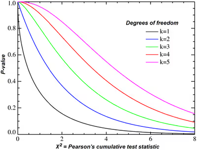
The test is valid when the test statistic is chi-squared distributed under the null hypothesis, specifically Pearson's chi-squared test and variants thereof. Pearson's chi-squared test is used to determine whether there is a statistically significant difference between the expected frequencies and the observed frequencies in one or more categories of a contingency table. For contingency tables with smaller sample sizes, a Fisher's exact test is used instead.

In the standard applications of this test, the observations are classified into mutually exclusive classes. If the null hypothesis that there are no differences between the classes in the population is true, the test statistic computed from the observations follows a χ² frequency distribution. The purpose of the test is to evaluate how likely the observed frequencies would be assuming the null hypothesis is true.

Test statistics that follow a χ² distribution occur when the observations are independent. There are also χ² tests for testing the null hypothesis of independence of a pair of random variables based on observations of the pairs.

Chi-squared tests often refers to tests for which the distribution of the test statistic approaches the χ² distribution asymptotically, meaning that the sampling distribution (if the null hypothesis is true) of the test statistic approximates a chi-squared distribution more and more closely as sample sizes increase.

History

In the 19th century, statistical analytical methods were mainly applied in biological data analysis and it was customary for researchers to assume that observations followed a normal distribution, such as Sir George Airy and Mansfield Merriman, whose works were criticized by Karl Pearson in his 1900 paper.

At the end of the 19th century, Pearson noticed the existence of significant skewness within some biological observations. To model the observations regardless of being normal or skewed, Pearson, in a series of articles published from 1893 to 1916, devised the Pearson distribution, a family of continuous probability distributions, which includes the normal distribution and many skewed distributions, and proposed a method of statistical analysis consisting of using the Pearson distribution to model the observation and performing a test of goodness of fit to determine how well the model really fits to the observations.

Pearson's chi-squared test

In 1900, Pearson published a paper on the χ² test which is considered to be one of the foundations of modern statistics. In this paper, Pearson investigated a test of goodness of fit.

Suppose that n observations in a random sample from a population are classified into k mutually exclusive classes with respective observed numbers of observations x_i (for i = 1,2,…,k), and a null hypothesis gives the probability p_i that an observation falls into the ith class. So we have the expected numbers m_i = np_i for all i, where

\begin{matrix} \sum_{i = 1}^{k} p_{i} = 1 \\ \sum_{i = 1}^{k} m_{i} = n \sum_{i = 1}^{k} p_{i} = n \end{matrix}

Pearson proposed that, under the circumstance of the null hypothesis being correct, as n → ∞ the limiting distribution of the quantity given below is the χ² distribution.

X^{2} = \sum_{i = 1}^{k} \frac{(x_{i} - m_{i})^{2}}{m_{i}} = \sum_{i = 1}^{k} \frac{x_{i}^{2}}{m_{i}} - n

Pearson dealt first with the case in which the expected numbers m_i are large enough known numbers in all cells assuming every observation x_i may be taken as normally distributed, and reached the result that, in the limit as n becomes large, X² follows the χ² distribution with k − 1 degrees of freedom.

However, Pearson next considered the case in which the expected numbers depended on the parameters that had to be estimated from the sample, and suggested that, with the notation of m_i being the true expected numbers and m′_i being the estimated expected numbers, the difference

X^{2} - {X^{'}}^{2} = \sum_{i = 1}^{k} \frac{x_{i}^{2}}{m_{i}} - \sum_{i = 1}^{k} \frac{x_{i}^{2}}{m_{i}^{'}}

will usually be positive and small enough to be omitted. In a conclusion, Pearson argued that if we regarded X′² as also distributed as χ² distribution with k − 1 degrees of freedom, the error in this approximation would not affect practical decisions. This conclusion caused some controversy in practical applications and was not settled for 20 years until Fisher's 1922 and 1924 papers.

6 more chapters are free with a Lably account.

Other examples of chi-squared tests

One test statistic that follows a chi-squared distribution exactly is the test that the variance of a normally distributed population has a given value based on a sample variance. Such tests are uncommon in practice because the true variance of the population is usually unknown. However, there are several statistical tests where the chi-squared distribution is approximately valid:

Fisher's exact test

For an exact test used in place of the 2 × 2 chi-squared test for independence when all the row and column totals were fixed by design, see Fisher's exact test. When the row or column margins (or both) are random variables (as in most common research designs) this tends to be overly conservative and underpowered.

Binomial test

For an exact test used in place of the 2 × 1 chi-squared test for goodness of fit, see binomial test.

Other chi-squared tests

Cochran–Mantel–Haenszel chi-squared test.
McNemar's test, used in certain 2 × 2 tables with pairing
Tukey's test of additivity
The portmanteau test in time-series analysis, testing for the presence of autocorrelation
Likelihood-ratio tests in general statistical modelling, for testing whether there is evidence of the need to move from a simple model to a more complicated one (where the simple model is nested within the complicated one).

Yates's correction for continuity

Using the chi-squared distribution to interpret Pearson's chi-squared statistic requires one to assume that the discrete probability of observed binomial frequencies in the table can be approximated by the continuous chi-squared distribution. This assumption is not quite correct and introduces some error.

To reduce the error in approximation, Frank Yates suggested a correction for continuity that adjusts the formula for Pearson's chi-squared test by subtracting 0.5 from the absolute difference between each observed value and its expected value in a 2 × 2 contingency table. This reduces the chi-squared value obtained and thus increases its p-value.

Chi-squared test for variance in a normal population

If a sample of size n is taken from a population having a normal distribution, then there is a result (see distribution of the sample variance) which allows a test to be made of whether the variance of the population has a pre-determined value. For example, a manufacturing process might have been in stable condition for a long period, allowing a value for the variance to be determined essentially without error. Suppose that a variant of the process is being tested, giving rise to a small sample of n product items whose variation is to be tested. The test statistic T in this instance could be set to be the sum of squares about the sample mean, divided by the nominal value for the variance (i.e. the value to be tested as holding). Then T has a chi-squared distribution with n − 1 degrees of freedom. For example, if the sample size is 21, the acceptance region for T with a significance level of 5% is between 9.59 and 34.17.

Example chi-squared test for categorical data

Suppose there is a city of 1,000,000 residents with four neighborhoods: A, B, C, and D. A random sample of 650 residents of the city is taken and their occupation is recorded as "white collar", "blue collar", or "no collar". The null hypothesis is that each person's neighborhood of residence is independent of the person's occupational classification. The data are tabulated as:

Let us take the sample living in neighborhood A, 150, to estimate what proportion of the whole 1,000,000 live in neighborhood A. Similarly we take ⁠349/650⁠ to estimate what proportion of the 1,000,000 are white-collar workers. By the assumption of independence under the hypothesis we should "expect" the number of white-collar workers in neighborhood A to be

150 \times \frac{349}{650} \approx 80.54

Then in that "cell" of the table, we have

\frac{{(observed - expected)}^{2}}{expected} = \frac{{(90 - 80.54)}^{2}}{80.54} \approx 1.11

The sum of these quantities over all of the cells is the test statistic; in this case, $\approx 24.57$ . Under the null hypothesis, this sum has approximately a chi-squared distribution whose number of degrees of freedom is

(number of rows - 1) (number of columns - 1) = (3 - 1) (4 - 1) = 6

If the test statistic is improbably large according to that chi-squared distribution, then one rejects the null hypothesis of independence.

A related issue is a test of homogeneity. Suppose that instead of giving every resident of each of the four neighborhoods an equal chance of inclusion in the sample, we decide in advance how many residents of each neighborhood to include. Then each resident has the same chance of being chosen as do all residents of the same neighborhood, but residents of different neighborhoods would have different probabilities of being chosen if the four sample sizes are not proportional to the populations of the four neighborhoods. In such a case, we would be testing "homogeneity" rather than "independence". The question is whether the proportions of blue-collar, white-collar, and no-collar workers in the four neighborhoods are the same. However, the test is done in the same way.

Applications

In cryptanalysis, the chi-squared test is used to compare the distribution of plaintext and (possibly) decrypted ciphertext. The lowest value of the test means that the decryption was successful with high probability. This method can be generalized for solving modern cryptographic problems.

In bioinformatics, the chi-squared test is used to compare the distribution of certain properties of genes (e.g., genomic content, mutation rate, interaction network clustering, etc.) belonging to different categories (e.g., disease genes, essential genes, genes on a certain chromosome etc.).

Limitations

The chi-squared test, while widely used for categorical data analysis, has several important limitations that researchers should consider. First, it assumes that observations are independent; violating this assumption can lead to misleading results. Second, the test is sensitive to sample size. In very large samples, even trivial differences between observed and expected frequencies may produce statistically significant results, while in very small samples, the test may lack power to detect meaningful associations. Third, the chi-squared test does not measure the strength or practical importance of an association—it only indicates whether a significant relationship exists. Effect size measures, such as Cramér's V or the contingency coefficient, should be reported alongside the test statistic to provide context. Finally, the test may be inaccurate when expected frequencies in any cell are very small, often recommended to be at least 5; in such cases, exact tests or alternative methods are preferred. Researchers must also be cautious when dealing with unevenly distributed categories, as dominant groups can overshadow patterns in smaller groups.