Random walk

An elementary example of a random walk is one on the integer number line ${\displaystyle \mathbb{Z}}$ which starts at 0, and at each step moves +1 or −1 with equal probability. Other examples include the path traced by a molecule as it travels in a liquid or a gas (see Brownian motion), the search path of a foraging animal, or the price of a fluctuating stock and the financial status of a gambler. Random walks have applications to engineering and many scientific fields including ecology, psychology, computer science, physics, chemistry, biology, economics, and sociology. The term random walk was first introduced by Karl Pearson in 1905.

Realizations of random walks can be obtained by Monte Carlo simulation.

In certain text, random walk is sometimes known as a drunkard's walk.

Lattice random walk

A popular random walk model is that of a random walk on a regular lattice, where at each step the location jumps to another site according to some probability distribution. In a simple random walk, the location can only jump to neighboring sites of the lattice, forming a lattice path. In a simple symmetric random walk on a locally finite lattice, the probabilities of the location jumping to each one of its immediate neighbors are the same. The best-studied example is the random walk on the d-dimensional integer lattice (sometimes called the hypercubic lattice) ${\displaystyle {\mathbb{Z}}^d}$. If, in addition, the state space is finite, the random walk model is called a simple bordered symmetric random walk, and the transition probabilities depend on the location of the state because on margin and corner states the movement is limited.

One-dimensional random walk

An elementary example of a random walk is the random walk on the integer number line, ${\displaystyle \mathbb{Z}}$, which starts at 0 and at each step moves +1 or −1 with equal probability.

This walk can be illustrated as follows. A marker is placed at zero on the number line, and a fair coin is flipped. If it lands on heads, the marker is moved one unit to the right. If it lands on tails, the marker is moved one unit to the left. After five flips, the marker could now be on -5, -3, -1, 1, 3, 5. With five flips, three heads and two tails, in any order, it will land on 1. There are 10 ways of landing on 1 (by flipping three heads and two tails), 10 ways of landing on −1 (by flipping three tails and two heads), 5 ways of landing on 3 (by flipping four heads and one tail), 5 ways of landing on −3 (by flipping four tails and one head), 1 way of landing on 5 (by flipping five heads), and 1 way of landing on −5 (by flipping five tails). See the figure below for an illustration of the possible outcomes of 5 flips.

To define this walk formally, take independent random variables ${\displaystyle Z_1,Z_2,\dots }$, where each variable is either 1 or −1, with a 50% probability for either value, and set ${\displaystyle S_0=0}$ and $S_n=\sum _{j=1}^n{Z}_j.$ The series ${\displaystyle \{S_n\}}$ is called the simple random walk on ${\displaystyle \mathbb{Z}}$. This series (the sum of the sequence of −1s and 1s) gives the net distance walked, if each part of the walk is of length one. The expectation ${\displaystyle E(S_n)}$ of ${\displaystyle S_n}$ is zero. That is, the mean of all coin flips approaches zero as the number of flips increases. This follows by the finite additivity property of expectation: $${\displaystyle E(S_n)=\sum _{j=1}^{n}E(Z_j)=0.}$$

A similar calculation, using the independence of the random variables and the fact that ${\displaystyle E(Z_n^2)=1}$, shows that: $${\displaystyle E(S_n^2)=\sum _{i=1}^{n}E(Z_i^2)+2\sum _{1\le i<j\le n}E(Z_i{Z}_j)=n.}$$

This hints that ${\displaystyle E(|S_n|)}$, the expected translation distance after n steps, should be of the order of ${\displaystyle \sqrt{n}}$. In fact, $${\displaystyle \underset{n\to \mathrm{\infty }}{lim}\frac{E(|S_n|)}{\sqrt{n}}=\sqrt{\frac{2}{\pi }}.}$$

To answer the question of how many times will a random walk cross a boundary line if permitted to continue walking forever, a simple random walk on ${\displaystyle \mathbb{Z}}$ will cross every point an infinite number of times. This result has many names: the level-crossing phenomenon, recurrence or the gambler's ruin. The reason for the last name is as follows: a gambler with a finite amount of money will eventually lose when playing a fair game against a bank with an infinite amount of money. The gambler's money will perform a random walk, and it will reach zero at some point, and the game will be over.

If a and b are positive integers, then the expected number of steps until a one-dimensional simple random walk starting at 0 first hits b or −a is ab. The probability that this walk will hit b before −a is ${\displaystyle a/(a+b)}$, which can be derived from the fact that simple random walk is a martingale. And these expectations and hitting probabilities can be computed in ${\displaystyle O(a+b)}$ in the general one-dimensional random walk Markov chain.

Some of the results mentioned above can be derived from properties of Pascal's triangle. The number of different walks of n steps where each step is +1 or −1 is 2ⁿ. For the simple random walk, each of these walks is equally likely. In order for S_n to be equal to a number k it is necessary and sufficient that the number of +1 in the walk exceeds those of −1 by k. It follows +1 must appear (n + k)/2 times among n steps of a walk, hence the number of walks which satisfy ${\displaystyle S_n=k}$ equals the number of ways of choosing (n + k)/2 elements from an n element set, denoted $(\genfrac{}{}{0ex}{}{n}{(n+k)/2})$. For this to have meaning, it is necessary that n + k be an even number, which implies n and k are either both even or both odd. Therefore, the probability that ${\displaystyle S_n=k}$ is equal to $2^{-n}(\genfrac{}{}{0ex}{}{n}{(n+k)/2})$. By representing entries of Pascal's triangle in terms of factorials and using Stirling's formula, one can obtain good estimates for these probabilities for large values of ${\displaystyle n}$.

This relation with Pascal's triangle is demonstrated for small values of n. At zero turns, the only possibility will be to remain at zero. However, at one turn, there is one chance of landing on −1 or one chance of landing on 1. At two turns, a marker at 1 could move to 2 or back to zero. A marker at −1, could move to −2 or back to zero. Therefore, there is one chance of landing on −2, two chances of landing on zero, and one chance of landing on 2.

The central limit theorem and the law of the iterated logarithm describe important aspects of the behavior of simple random walks on ${\displaystyle \mathbb{Z}}$. In particular, the former entails that as n increases, the probabilities (proportional to the numbers in each row) approach a normal distribution.

To be precise, knowing that $\mathbb{P}(X_n=k)=2^{-n}(\genfrac{}{}{0ex}{}{n}{(n+k)/2})$, and using Stirling's formula one has

$${\displaystyle \log \mathbb{P}(X_n=k)=n\left[\left(1+\frac{k}{n}+\frac{1}{2n}\right)\log \left(1+\frac{k}{n}\right)+\left(1-\frac{k}{n}+\frac{1}{2n}\right)\log \left(1-\frac{k}{n}\right)\right]+\log \frac{\sqrt{2}}{\sqrt{\pi }}+o(1).}$$

Fixing the scaling $k=\lfloor \sqrt{n}x\rfloor$, for $x$ fixed, and using the expansion $\log (1+k/n)=k/n-k^2/2n^2+\dots$ when $k/n$ vanishes, it follows

$${\displaystyle \mathbb{P}\left(\frac{X_n}{n}=\frac{\lfloor \sqrt{n}x\rfloor }{\sqrt{n}}\right)=\frac{1}{\sqrt{n}}\frac{1}{2\sqrt{\pi }}{e}^{-x^2}(1+o(1)).}$$

taking the limit (and observing that $1/\sqrt{n}$ corresponds to the spacing of the scaling grid) one finds the gaussian density $f(x)=\frac{1}{2\sqrt{\pi }}{e}^{-x^2}$. Indeed, for a absolutely continuous random variable $X$ with density $f_X$ it holds $\mathbb{P}\left(X\in [x,x+dx)\right)=f_X(x)dx$, with $dx$ corresponding to an infinitesimal spacing.

As a direct generalization, one can consider random walks on crystal lattices (infinite-fold abelian covering graphs over finite graphs). Actually it is possible to establish the central limit theorem and large deviation theorem in this setting.

As a Markov chain

A one-dimensional random walk can also be looked at as a Markov chain whose state space is given by the integers ${\displaystyle i=0,\pm 1,\pm 2,\dots .}$ For some number p satisfying ${\displaystyle 0<p<1}$, the transition probabilities (the probability P_i,j of moving from state i to state j) are given by $${\displaystyle P_{i,i+1}=p=1-P_{i,i-1}.}$$

Heterogeneous generalization

The heterogeneous random walk draws in each time step a random number that determines the local jumping probabilities and then a random number that determines the actual jump direction. The main question is the probability of staying in each of the various sites after ${\displaystyle t}$ jumps, and in the limit of this probability when ${\displaystyle t}$ is very large.

Higher dimensions

In higher dimensions, the set of randomly walked points has interesting geometric properties. In fact, one gets a discrete fractal, that is, a set which exhibits stochastic self-similarity on large scales. On small scales, one can observe "jaggedness" resulting from the grid on which the walk is performed. The trajectory of a random walk is the collection of points visited, considered as a set with disregard to when the walk arrived at the point. In one dimension, the trajectory is simply all points between the minimum height and the maximum height the walk achieved (both are, on average, on the order of ${\displaystyle \sqrt{n}}$).

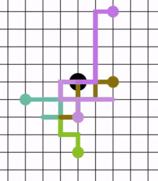
To visualize the two-dimensional case, one can imagine a person walking randomly around a city. The city is effectively infinite and arranged in a square grid of sidewalks. At every intersection, the person randomly chooses one of the four possible routes (including the one originally travelled from). Formally, this is a random walk on the set of all points in the plane with integer coordinates.

To answer the question of the person ever getting back to the original starting point of the walk, this is the 2-dimensional equivalent of the level-crossing problem discussed above. In 1921 George Pólya proved that the person almost surely would in a 2-dimensional random walk, but for 3 dimensions or higher, the probability of returning to the origin decreases as the number of dimensions increases. In 3 dimensions, the probability decreases to roughly 34%. The mathematician Shizuo Kakutani was known to refer to this result with the following quote: "A drunk man will find his way home, but a drunk bird may get lost forever".

The probability of recurrence is in general ${\displaystyle p=1-{\left(\frac{1}{(2\pi {)}^d}{\int }_{[-\pi ,\pi {]}^d}\frac{\prod _{i=1}^{d}d{\theta }_i}{1-\frac{1}{d}\sum _{i=1}^d\cos {\theta }_i}\right)}^{-1}}$, which can be derived by generating functions or Poisson process.

Another variation of this question which was also asked by Pólya is: "if two people leave the same starting point, then will they ever meet again?" It can be shown that the difference between their locations (two independent random walks) is also a simple random walk, so they almost surely meet again in a 2-dimensional walk, but for 3 dimensions and higher the probability decreases with the number of the dimensions. Paul Erdős and Samuel James Taylor also showed in 1960 that for dimensions less or equal than 4, two independent random walks starting from any two given points have infinitely many intersections almost surely, but for dimensions higher than 5, they almost surely intersect only finitely often.

The asymptotic function for a two-dimensional random walk as the number of steps increases is given by a Rayleigh distribution. The probability distribution is a function of the radius from the origin and the step length is constant for each step. Here, the step length is assumed to be 1, N is the total number of steps and r is the radius from the origin.

$${\displaystyle P(r)=\frac{2r}{N}{e}^{-r^2/N}}$$

Relation to Wiener process

A Wiener process is a stochastic process with similar behavior to Brownian motion, the physical phenomenon of a minute particle diffusing in a fluid. (Sometimes the Wiener process is called "Brownian motion", although this is strictly speaking a confusion of a model with the phenomenon being modeled.)

A Wiener process is the scaling limit of random walk in dimension 1. This means that if there is a random walk with very small steps, there is an approximation to a Wiener process (and, less accurately, to Brownian motion). To be more precise, if the step size is ε, one needs to take a walk of length L/ε² to approximate a Wiener length of L. As the step size tends to 0 (and the number of steps increases proportionally), random walk converges to a Wiener process in an appropriate sense. Formally, if B is the space of all paths of length L with the maximum topology, and if M is the space of measure over B with the norm topology, then the convergence is in the space M. Similarly, a Wiener process in several dimensions is the scaling limit of random walk in the same number of dimensions.

A random walk is a discrete fractal (a function with integer dimensions; 1, 2, ...), but a Wiener process trajectory is a true fractal, and there is a connection between the two. For example, take a random walk until it hits a circle of radius r times the step length. The average number of steps it performs is r². This fact is the discrete version of the fact that a Wiener process walk is a fractal of Hausdorff dimension 2.

In two dimensions, the average number of points the same random walk has on the boundary of its trajectory is r^4/3. This corresponds to the fact that the boundary of the trajectory of a Wiener process is a fractal of dimension 4/3, a fact predicted by Mandelbrot using simulations but proved only in 2000 by Lawler, Schramm and Werner.

A Wiener process enjoys many symmetries a random walk does not. For example, a Wiener process walk is invariant to rotations, but the random walk is not, since the underlying grid is not (random walk is invariant to rotations by 90 degrees, but Wiener processes are invariant to rotations by, for example, 17 degrees too). This means that in many cases, problems on a random walk are easier to solve by translating them to a Wiener process, solving the problem there, and then translating back. On the other hand, some problems are easier to solve with random walks due to its discrete nature.

Random walk and Wiener process can be coupled, namely manifested on the same probability space in a dependent way that forces them to be quite close. The simplest such coupling is the Skorokhod embedding, but there exist more precise couplings, such as Komlós–Major–Tusnády approximation theorem.

The convergence of a random walk toward the Wiener process is controlled by the central limit theorem, and by Donsker's theorem. For a particle in a known fixed position at t = 0, the central limit theorem tells us that after a large number of independent steps in the random walk, the walker's position is distributed according to a normal distribution of total variance:

$${\displaystyle {\sigma }^2=\frac{t}{\delta t}{\epsilon }^2,}$$

where t is the time elapsed since the start of the random walk, ${\displaystyle \epsilon }$ is the size of a step of the random walk, and ${\displaystyle \delta t}$ is the time elapsed between two successive steps.

This corresponds to the Green's function of the diffusion equation that controls the Wiener process, which suggests that, after a large number of steps, the random walk converges toward a Wiener process.

In 3D, the variance corresponding to the Green's function of the diffusion equation is: $${\displaystyle {\sigma }^2=6Dt.}$$

By equalizing this quantity with the variance associated to the position of the random walker, one obtains the equivalent diffusion coefficient to be considered for the asymptotic Wiener process toward which the random walk converges after a large number of steps: $${\displaystyle D=\frac{{\epsilon }^2}{6\delta t}}$$ (valid only in 3D).

The two expressions of the variance above correspond to the distribution associated to the vector ${\displaystyle \overrightarrow{R}}$ that links the two ends of the random walk, in 3D. The variance associated to each component ${\displaystyle R_x}$, ${\displaystyle R_y}$ or ${\displaystyle R_z}$ is only one third of this value (still in 3D).

For 2D:

$${\displaystyle D=\frac{{\epsilon }^2}{4\delta t}.}$$

For 1D:

$${\displaystyle D=\frac{{\epsilon }^2}{2\delta t}.}$$